Conditional Expectation Functions and Regression
EC655 - Econometrics
Justin Smith
Wilfrid Laurier University
Fall 2023

Introduction
Introduction
Questions in economics often involve explaining a variable in terms of others
Does age of school entry affect test scores?
Does childhood health insurance affect adult health?
Does foreign competition affect domestic innovation?
Interest is usually in the causal relationship
- The independent effect of one variable on another
Econometrics provides a framework for examining these relationships
- Strong focus on causality
What Are We Trying To Model?
Conditional Expectation Function
We want to relate dependent variable \(y\) to independent variables \(\mathbf{x}\)
Want to know systematically what happens to \(y\) when \(\mathbf{x}\) changes
Difficult because \(y\) and \(\mathbf{x}\) are random variables
- \(y\) can take many different values for each \(\mathbf{x}\)
A way systematic patterns is to focus on average \(y\) at each \(\mathbf{x}\)
- Ex: Does average achievement fall as we increase class size?
This is the conditional expectation function (CEF) \(\mathbf{E}[y|\mathbf{x}]\)
Note
The CEF is the population average value of \(y\) at each \(\mathbf{x}\). The average can change at different \(\mathbf{x}\), meaning it is a function of \(\mathbf{x}\).
Conditional Expectation Function
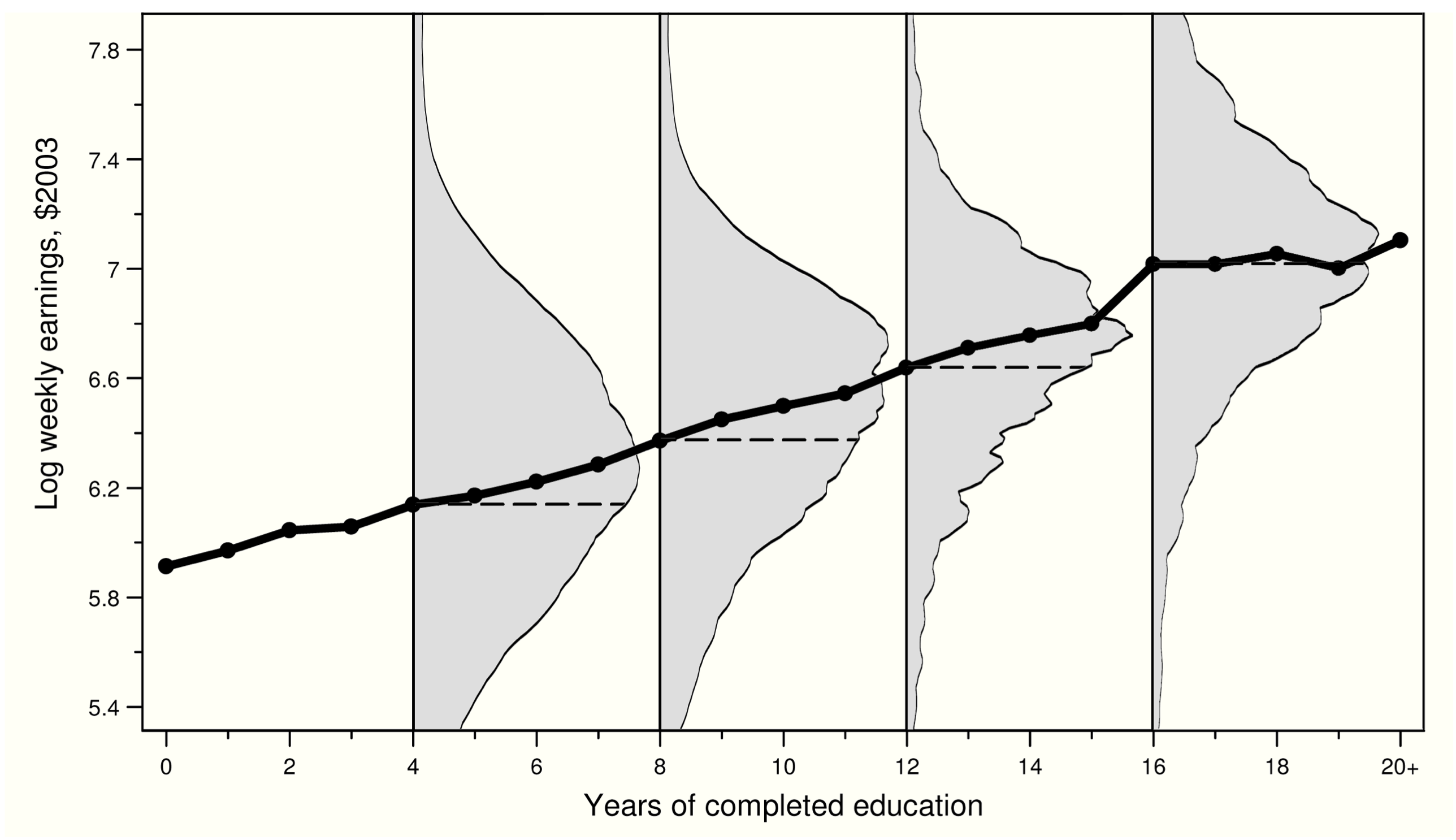
Log earnings on vertical axis, years of schooling on horizontal
Grey shaded areas are distribution of log earnings at each level of schooling
- Big spread incomes for each level of schooling
Black line is the CEF of earnings at each level of schooling
- Increasing pattern between school and earnings is easier to see
Conditional Expectation Function
The CEF highlights the pattern through randomness
It is the optimal predictor of \(y\) given \(\mathbf{x}\)
- It minimizes the mean squared error in predicting \(y\)
Problem with using CEF: as a population value, it is not known
- It is not observable because we do not see the population
Instead, use linear regression to approximate it
Linear Regression
Motivation
We can use linear regression to approximate CEF. Why?
If the CEF is linear, it is equivalent to population regression function
The population regression function is the best linear predictor of \(y\) given \(\mathbf{x}\)
The population regression function is the best linear approximation to the CEF
This is partly why linear regression is popular in economics
Next section examines population regression
- We will cover estimation of the population regression with a sample later
Note
Most undergrad classes do not derive the population regression slope and instead skip directly to estimation with a sample, so this may be new. It is important to understand that at this point there is no data; we are only talking about features of the population. As you will see later, the population and sample regression functions are closely related.
Population Regression Function
- A linear model relating \(y\) to explanatory variables \(\mathbf{x}\) is
\[y = \mathbf{x}\boldsymbol{\beta} + u\]
Where
\(y\) is a scalar observable random outcome variable
\(\mathbf{x}\) is a \(1\times (k + 1)\) vector of random explanatory factors
\(\boldsymbol{\beta}\) is a \((k + 1) \times 1\) vector of slope parameters (non-random)
\(u\) is a scalar population residual term
\(\mathbf{x}\boldsymbol{\beta}\) is called the Population Regression Function (PRF)
- The part of \(y\) that is predictable by \(\mathbf{x}\)
Population Regression Function
Use the PRF to approximate the CEF
If CEF is linear, PRF equals CEF
- True when model is “saturated” or when variables are joint Normal
Still useful to use PRF if CEF is not linear
- Goal is capture essential features of relationship
Saturated Models
A saturated model is one where the independent variables are discrete, and there is a dummy variable for each possible value it can take. For example if you regress wages on gender, a (saturated) CEF is
\[E[wage|female] = \alpha + \beta female\]
where \(\alpha = E[wage|female = 0]\) and \(\beta =E[wage|female = 1] - E[wage|female = 0]\)
Population Regression Slope Vector
- The population least squares vector minimizes the mean squared prediction error (MSPE)
\[\min_\beta \textbf{E}[(y-\mathbf{x}\boldsymbol{\beta})^2]\]
- Take the derivative with respect to \(\boldsymbol{\beta}\) to get first order condition
\[\textbf{E}[\mathbf{x}'(y-\mathbf{x}\boldsymbol{\beta})]= \mathbf{0}\]
- Solve for \(\boldsymbol{\beta}\)
\[\textbf{E}[\mathbf{x}'y]= \textbf{E}[\mathbf{x'x}\boldsymbol{\beta}]\] \[\textbf{E}[\mathbf{x}'y]= \textbf{E}[\mathbf{x'x}]\boldsymbol{\beta}\] \[(\textbf{E}[\mathbf{x'x}])^{-1} \textbf{E}[\mathbf{x}'y]= \boldsymbol{\beta}\]
Population Regression Slope Vector
Important
The population least squares slope vector is
\[\boldsymbol{\beta} = (\textbf{E}[\mathbf{x'x}])^{-1} \textbf{E}[\mathbf{x}'y]\]
- Now consider pulling the intercept out of the \(\boldsymbol{\beta}\) vector
\[y = \alpha + \mathbf{x}\boldsymbol{\beta} + u\]
- Take the mean of this equation
\[E[y] = E[\alpha + \mathbf{x}\boldsymbol{\beta} + u] = \alpha + E[\mathbf{x}]\boldsymbol{\beta}\]
Population Regression Slope Vector
- Subtract from first equation
\[y - E[y] = (\mathbf{x}\boldsymbol - E[\mathbf{x}]){\beta} + u\]
- Using the population linear regression vector formula
\[\boldsymbol{\beta} = (\textbf{E}[\mathbf{(\mathbf{x}\boldsymbol - \textbf{E}[\mathbf{x}])'(\mathbf{x}\boldsymbol - \textbf{E}[\mathbf{x}])}])^{-1} \textbf{E}[(\mathbf{x}\boldsymbol - \textbf{E}[\mathbf{x}])'(y - \textbf{E}[y])] = VAR[\mathbf{x}]^{-1}COV[\mathbf{x},y]\]
Important
An alternative way to write the population least squares vector is
\[\boldsymbol{\beta} = VAR[\mathbf{x}]^{-1}COV[\mathbf{x},y]\]
\[\alpha = \textbf{E}[y] - \textbf{E}[\mathbf{x}]\boldsymbol{\beta}\]
Properties of Population Regression
- The first order condition from minimizing the MSPE by choosing \(\boldsymbol{\beta}\) is
\[\textbf{E}[\mathbf{x}'(y-\mathbf{x}\boldsymbol{\beta})]= \mathbf{0}\]
- This is the same as saying
\[\textbf{E}[\mathbf{x}'u]=\mathbf{0}\]
- Expanding that equation, we get
\[\begin{bmatrix} \textbf{E}(u)\\ \textbf{E}(x_{1}u)\\ \vdots\\ \textbf{E}(x_{k}u) \end{bmatrix} =\mathbf{0}\]
Properties of Population Regression
\(\textbf{E}[\mathbf{x}'u]=\mathbf{0}\) says two important things
The average value of the population residual \(u\) is zero
The covariance between each \(x\) and \(u\) is zero
To see the covariance part
\[\text{cov}(x_{1},u) = \mathbf{E}[(x_{1} - \mathbf{E}(x_{1}))(u - \mathbf{E}(u))]\]
- From above, we know that \(\mathbf{E}(u) =0\), so
\[\text{cov}(x_{1},u) = \mathbf{E}[x_{1}u - \mathbf{E}(x_{1})u]\]
Population Regression Slope Vector
- Bringing the expectation through the brackets
\[\text{cov}(x_{1},u) = \mathbf{E}(x_{1}u) - \mathbf{E}(x_{1})\mathbf{E}(u) = \mathbf{E}(x_{1}u)\]
- Says that \(u\) is mean zero and uncorrelated with \(\mathbf{x}\)
Note
\(u\) is the population residual, and is defined as \(u = y - \mathbf{x}\boldsymbol{\beta}\) where \(\boldsymbol{\beta} = (\textbf{E}[\mathbf{x'x}])^{-1} \textbf{E}[\mathbf{x}'y]\)
By definition it has mean zero and is uncorrelated with \(\mathbf{x}\). We cannot use this to determine causality, which is determined by whether the slope in the CEF has a causal interpretation. We will discuss this in detail later.
Example 1: Joint Normal Variables
Linear CEF and Regression
There are two special cases when the CEF is definitely linear
Joint Normal variables
Saturated models
We show below that in these cases the PRF and the CEF are identical
Note again that we have no data yet
- We are just comparing features of the population
Joint Normal Variables
Suppose the random variables \(y\) and \(x\) have a bivariate Normal distribution
The CEF of \(y\) given \(x\) is
\[ E[y|x] = \mu_{y} + \rho \frac{\sigma_{y}}{\sigma_{x}}(x - \mu_{x}) \]
The terms in this equation are
- \(\mu_{x}, \mu_{y}\) are the population means of \(x,y\)
- \(\sigma_{x}, \sigma_{y}\) are the population standard deviations of \(x,y\)
- \(\rho\) is the correlation coefficient between \(x,y\)
This is linear in \(x\) with slope \(\rho \frac{\sigma_{y}}{\sigma_{x}}\)
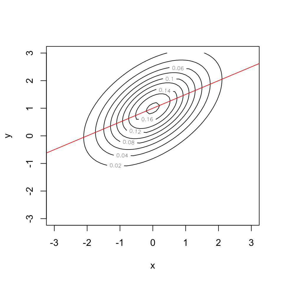
Joint Normal Variables
Keep things simple and assume
- \(\mu_{x} = 0\) and \(\mu_{y} = 1\)
- \(\sigma_{x} = 1\) and \(\sigma_{y} = 1\)
- \(\rho = 0.5\)
In this example the CEF is
\[ E[y|x] = 1 + 0.5x \]
Distribution Plot
Estimating The CEF with PRF
- The population regression equation to estimate this CEF would be
\[y = \alpha + x\beta + u\]
- We derived that the slope in this regression is
\[\beta = \frac{cov(x,y)}{var(x)}\]
From previous slide we know
- \(var(x) = 1\)
- \(cov(x,y) = \rho \sigma_{x} \sigma_{y} = 0.5\)
The population slope value is therefore \(\beta = 0.5\), exactly the slope of the CEF
The intercept is \(\alpha = \mu_{y} - \mu_{x}\beta = 1\)
Example 2: Saturated Model
CEF with Binary Regressor
Imagine that \(y\) is a continuous variable, and \(x\) takes on two values \((0,1)\)
The CEF for these variables is
\[E[y|x] = E[y|x = 0] + (E[y|x=1] -E[y|x=0])x\] \[ = \alpha + \beta x\]
- The slope is the difference in means between the two groups
Population Regression Function
- Again, the population regression is
\[y = \alpha + x\beta + u\]
- Taking expectations we get
\[E[y|x=0] = \alpha + E[u|x = 0]\] \[E[y|x=1] = \alpha + \beta + E[u|x = 1]\]
- The difference is
\[E[y|x=1] - E[y|x=0] = \beta + E[u|x = 1] - E[u|x = 0]\]
Population Regression Function
The last two terms are zero because of the properties of regression
To see this recall that \(E[u] = 0\) in regression, and the Law of Iterated Expectations means
\[E[xu] = E[xE[u|x]] = 0\]
- Since \(x\) takes two values, the only way for this to be true is
\[ E[u|x = 1] =E[u|x = 0] = 0\]
- This means
\[\beta = E[y|x=1] - E[y|x=0]\]
- This is exactly the same value as the CEF
Example 3: Non-linear CEF
CEF
The CEF and PRF are not equal when the CEF is non-linear
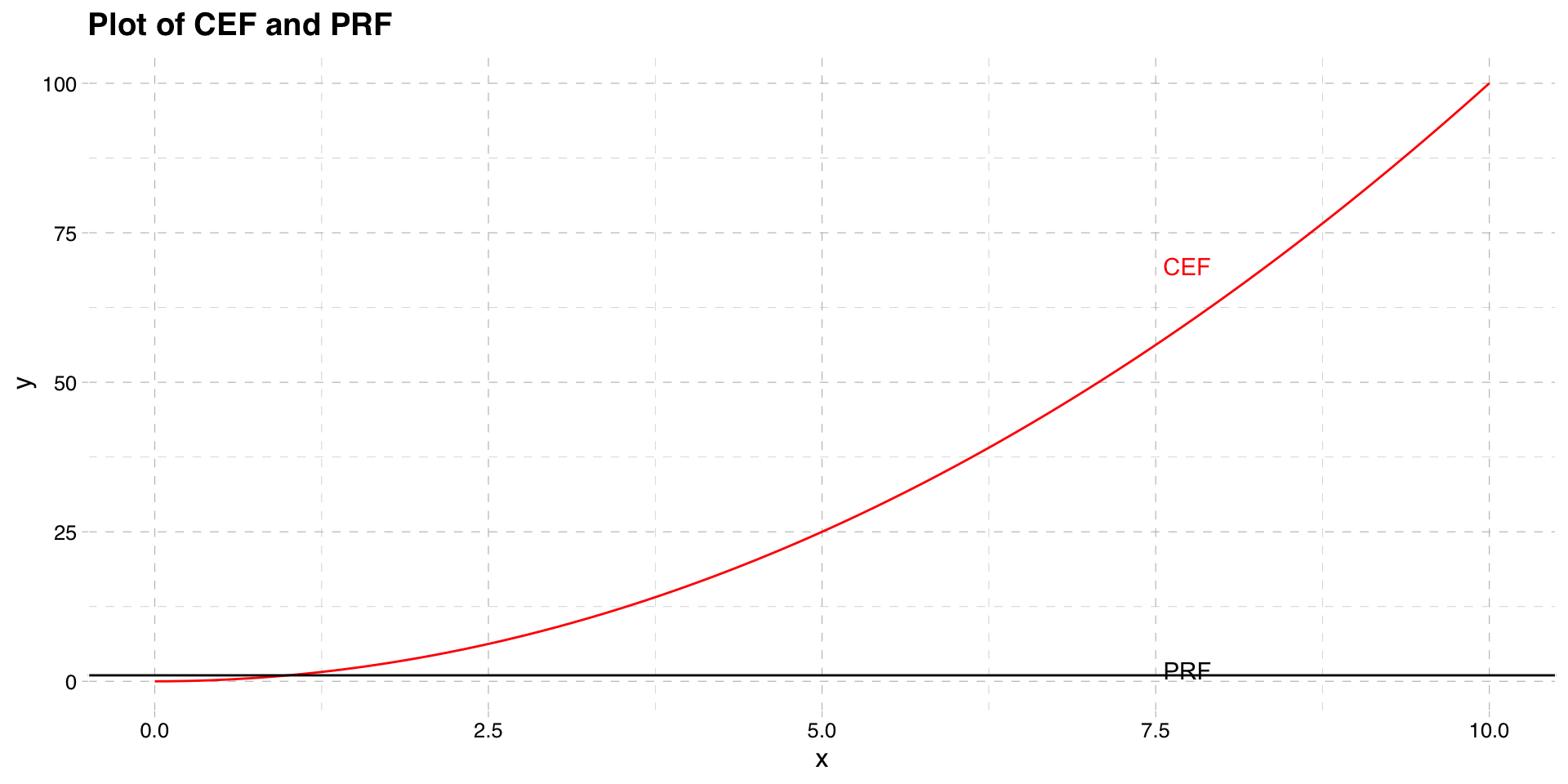
Suppose that the random variable y is determined by
\[y = x^2 + \epsilon\]
Assume the variable \(x \sim \mathcal{N}(0, 1)\) and \(\epsilon \sim \mathcal{N}(0, 1)\) and independent of \(x\)
The non-linear CEF in this setup is
\[E[y|x] = x^2\]
Caution
The random variable \(\epsilon\) is not the same as the regression residual \(u\). The residual \(u\) is defined as \(u = y- x\beta\), whre \(\beta\) is the population regression slope vector. In this example, you can think of \(\epsilon\) as just another random variable, like \(x\).
Population Regression
- A linear regression function would specify the relationship as
\[y = \alpha + x\beta + e\]
- We know the population slope is
\[\beta = \frac{cov(x,y)}{var(x)}\]
Because \(x \sim \mathcal{N}(0, 1)\) we know \(var(x) = 1\)
The covariance term is calculated as
\[cov(x,y) = cov(x, x^2 + \epsilon)\] \[=cov(x,x^2) + cov(x,\epsilon)\]
Population Regression
The second term is zero because \(x\) and \(\epsilon\) are independent
For Standard Normal random variables, \(x\) and \(x^2\) are also uncorrelated
Based on this, the PRF slope is
\[\beta = 0\]
- The population intercept is
\[\alpha = E[y] - E[x]\beta\] \[=E[x^2 + \epsilon] - E[x]\beta\] \[=1\]
Graphical Comparison
Summary
What did we learn?
In econometrics we are often interested in how variables are related
To do this, we study how the mean of one variable changes with another
We mostly do not know the mean function, so approximate it with regression
In population regression the slope vector minimizes the MSPE
Regression residuals are by definition mean zero and unrelated to \(\mathbf{x}\)
So far we have only discussed this in the population
- Use of data is coming later